Now that we have discussed the two experiments needed to lay the groundwork for the quantum physics involved here and here, we can move on to the first principle used in quantum computers: superposition. If at any point you need a refresher, click on those two links above to learn more about the polarization experiment and the double-slit experiment.

The Start of a Quantum Revolution, Through a Double-Slit

Our previous post overviewed the double-slit experiment’s history, development, and meaning. Here, we will dive deeper into the experiment and demonstrate the actual nature and mechanics involved with superposition.

As we did there, we can start here with Isaac Newton. By the turn of the 18th century, Newton developed and published his theory of light composed of particles, the “corpuscular theory.” We won’t dig further into that theory for now. Still, the point of including it here is that over the next two centuries, arguments developed over the nature of light: one side argued that it was composed of waves, while the other argued that it was composed of particles.

Thomas Young created his experiment to demonstrate and support the argument that light was composed of waves. By the time of his experiment, though, scientific giants like Robert Hooke, Christiaan Huygens, and Augustin-Jean Fresnel had developed the mathematics that would support the propagation of light waves. As such, Young’s experiment sought to demonstrate such principles in action physically.

The double-slit experiment Young came up with is quite simple and has been repeated by scientists with different mediums and different environments. The original involves a light shined towards two screens, one placed in front of the other. The first screen has two slits placed in it, through which the light filters through and creates a pattern on the second screen.

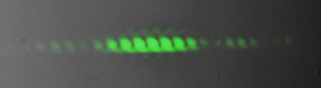
Starting from one slit being closed, the pattern that appears on the second screen is exactly what you would expect: a bright line. When both slits are open, the light starts acting in peculiar ways. The pattern that emerges on the back screen does not look like light filtering through two vertical slits: it instead shows alternating lines of light and dark across the screen.

The emerging pattern, seen in the second image above, has become known as an “interference pattern.” The reason for this is that the pattern that emerges — rather than lining up with the slits — demonstrates that light traveling towards the first screen splits into two new waves. The waves recreate themselves and start to spread again towards the second screen. The waves then come into contact with each other, creating different types of interference depending on where the waves come into contact with each other.

If they come into contact with each other at their peaks or troughs, they create a brighter section of light on the back screen due to “constructive interference” (constructive because the two waves meeting at their peak or trough amplify the resulting wave). If the waves come into contact with each other when one is at its peak and the other is at its trough (or some variation thereof), the two waves cancel out, creating a darker pattern as a result of “destructive interference” (destructive because the waves cancel each other out). One can then determine how the light waves interfered with each other based on the resulting “interference pattern.”

While it would seem that the experiment confirmed Young and company’s light-as-wave argument, alterations to the experiment over the twentieth century and Einstein’s photoelectric effect experiments would show that the photons would also have particle characteristics. We can jump into Einstein’s experiment first and then detail how scientists throughout the twentieth century demonstrated photons have both particle and wave-like characteristics.

In 1905, Einstein demonstrated that light can behave like it is composed of particles by shining light onto a metal surface. By changing the energy levels of the light by changing the light frequency, the lights hits the metal surface and ejects electrons, creating further energy. The energy and number of electrons ejected change depending on the frequency as long as the frequency is above a threshold frequency.

Einstein’s publication detailing the experiment explained it by first proposing that light was composed of discrete particles called “photons.” Each photon, in turn, has energy proportional to the light frequency; he described such a relationship with the equation E = hf, with E being the energy, h being Planck’s constant, and f being the light frequency. When the photon hits the metal surface — i.e., when it hits the electrons in the metal surface — the photon transfers the energy contained within it to the electron. This is where the threshold items comes in: if the photon’s energy exceeds the base energy required to remove an electron from the metal, the electron is ejected. Because this relationship depends on the intensity of the light, which entails more photons, the transfer demonstrates that the photons had particle-like characteristics.

Further alterations to the double-slit experiment supported the growing evidence of photons having wave and particle characteristics. As the twentieth century progressed, so too did the devices that could be used to control the flow of light to screens. The scientific community recognized by that point that if they replaced the light with some composed of particles — sand, for example — the pattern appearing on the back screen would follow the common sense model: two lines parallel to the slits. However, when the experimenter changed the device sending the light to the screens, allowing the tester to control the amount of light sent and the interval between each light particle, a new picture emerged.

Now, the experimenter controlled the interval and the amount of light sent to the screens. At first, the pattern that emerged on the second screen suggested particle patterns. Over time, though, the interference patterns first witnessed by Young emerged, even though the amount of light sent to the screens was limited, and intervals were established between each round of light sent.

To be clear, we want to make sure you see how weird this is: single quanta of light were fired at the first screen, giving enough time for it to hit both screens before the next light was sent. And still, the interference pattern emerged. This suggested that the photon was breaking itself apart, going through both slits, reemerging from the other side where it hit the other electron, and creating interference before creating the corresponding pattern on the second screen.

One photon has a wave-like property when fired through a double-slit; the same photon transfers electrons to another material’s electrons. The different maker between the two is how the experimenter measured or observed the particle: passing through slits, they can be observed acting like waves. Reflecting off a metal surface, they act like particles. The theoretical and mechanical result? Wave-particle duality, the subject of our next section.

Wave-Particle Duality

What is wave-particle duality? In a sense, we explained it by describing the double-slit experiment and Einstein’s discovery of the photoelectric effect: photons can act like waves and particles. And as we’ll see in this and the coming section, they can be both simultaneously.

For now, though, we will only treat the wave-particle duality in terms of the photon or other particle having wave-like characteristics one moment and particle-like the next. Whether the quantum matter will have wave-like or particle-like characteristics depends on the measurement method or observation.

Scientists can determine the nature of both wave-like and particle-like characteristics using mathematical methods developed by two of the field’s giants: Erwin Schrödinger and Albert Einstein. As we’ve described the mechanics going on with particles in the last section (E = hf), we can not detail the photon’s wave characteristics.

To contextualize this before diving further into it, we can demonstrate that photons act like waves based solely on the interference pattern alone: only through waves coming together and interfering with each other can the interference pattern be made. Constructive and destructive interference are wave characteristics of photons. We here are now talking about properties such as location, probability of the photon being a particle or wave, speed, etc. When scientists discuss these traits, they talk about information governed by the wave function, which is governed by the Schrödinger equation.

The Wave Function and Schrödinger Equation

We will warn you that this section is going to be math-heavy. To fully understand why the wave function and Schrödinger equation are essential, you must understand most of the mathematics. If you don’t want to learn the mathematics, you will be missing out, but you can skip to the end of the section, where we summarize the essential parts and contextualize everything.

The wave function is a mathematical function that determines the probabilities of finding a photon or other quantum matter in a particular state upon measurement. The wave function is arrived at by solving the Schrödinger equation; the solution is represented using the Greek letter Psi (Ψ). Because the wave function is a probability, it is usually expressed in its squared form (|Ψ|²), which shows a probability density of finding the quantum matter at that particular location in space at a given time.

As mentioned, solving the Schrödinger equation arrives at the wave function. This is where the description will get particularly math-heavy: the Schrödinger equation is a linear partial differential equation that can provide information about the quantum matter. Let’s break it down further.

A “linear partial differential equation” is a head-spinner of a term. What it means is that the Schrödinger equation is an equation that can be used to find unknown functions by taking partial derivatives of a function that is composed of several variables. It should be noted that depending on the variables involved and the variables or functions that one is trying to determine using the equation, there may be multiple solutions. If this is the case, a combination of such solutions is also a valid solution.

Take a moment here before we provide more details on the equation, and pay attention to that last sentence. Multiple solutions are valid if they are made by combining valid solutions. This is a baseline definition of linearity and a baseline characteristics of superposition.

There are two types of Schrödinger equations, depending on whether the use of the equation considers time measurements. As such, the first of these — the time-dependent Schrödinger equation — is the one that provides the most information about the quantum matter in question. The second type — the time-independent Schrödinger equation — is a simplified version of the time-dependent equation that does not provide information about how time is figured into the equation, i.e., how the system changes over time.

Due to this simplified nature, let’s jump into the time-dependent Schrödinger equation (TDSE). A solution of the TDSE will provide a wave function whose information includes how the quantum matter in question changes over time. This includes position, change in position, time, etc. Here is the equation for the time-dependent Schrödinger equation:

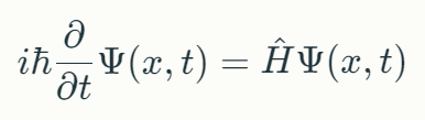
Walking through this equation, we see first an imaginary unit, symbolized by i. The ℏ is the reduced Planck’s constant, Ψ (x, t) is the wavefunction that the equation will solve while x and t are position and time (hence, the wavefunction is dependent on position and time). Next is Ĥ, which refers to the Hamiltonian unit, an operator that provides the system’s total energy. It is important to note that because the time-dependent Schrödinger equation essentially describes how the system changes over time, the energy accounted for can be both potential and kinetic.

The time-independent Schrödinger equation (TISE) is when the Hamiltonian operator does not depend on time, i.e., the system’s energy remains constant. This equation is often used to find just the energy levels of corresponding wavefunctions, which can then be used to determine a system’s spatial distribution. The time-independent Schrödinger equation is given by:

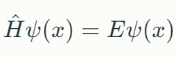
Here we see the Hamiltonian operator is still taken into consideration as is the wave function, ψ. Note that because this wave function relies on position (and not time), it is reflected using the lowercase psi. On the other side of the equal sign, E is the energy eigenvalue associated with the wave function at a particular position.

We can gather the information, enter it into the equation, and determine the wave function. By squaring the wave function, we can find a probability density of finding a particular piece of quantum matter at a specific location at a certain time in a particular state.

Bringing It Around and Bringing In Superposition

Where does this all fit into the overall topic? Now that we know the mathematics, we can dive into what we are talking about when we discuss superposition.

We showed previously that in the double-slit experiment, the pattern created on the second screen would demonstrate the photon acting like a particle at certain times and waves at other times. This is the wave-particle duality; the mechanics of how they will interact are given by equations that demonstrate the photoelectric effect for particles (E = hf) and the wave function/

We showed previously that in the double-slit experiment, the pattern created on the second screen would demonstrate the photon acting like a particle at certain times and waves at other times. This is the wave-particle duality; the mechanics of how they will interact are given by equations that demonstrate the photoelectric effect for particles (E = hf) and the wave function/Schrödinger equation for waves, whether the photon will act as a particle or a wave depend on the way we are measuring or observing the photon. Just remember this and the mathematics because what is occurring is weird to read in words.

Even if we assumed that the photon going through the two slits did so as a wave, we could assume that there would be two grouped patterns on the screen. The varying shades of the interference pattern, made of alternating lighter and darker areas based on the interference in question, show that they are going through as waves. However, because the interference pattern develops when the photons are sent through one at a time, it acts as a wave (based on the interference pattern) but interferes with itself. In other words, it is going through both of the slits at the same time. Not only that but according to the Schrödinger equation and wave function, it could go through every possible path to the screen, again, at the same time.

This means the experiment and the mathematics demonstrate the photons can be in multiple positions at the same time. The photon is also both wave and particle at the same time. It will only go to a certain location and collapse to a certain state when measured or observed. However, we can’t know that state until we measure it, but we can base it on probabilities, hence the probabilistic nature of the wave function.

A Summary, a Link to Quantum Computers, and a Conclusion

So, let’s recap. The mathematics, the double-slit experiments, and Einstein’s description of the photoelectric effect all demonstrate that photons and other quantum matter can have wave and particle characteristics (i.e., wave-particle duality). The particle nature is governed by equations like Einstein’s photoelectric effect equation (E = hf). In contrast, the wave characteristics are governed by the Schrödinger equation, which can give the probabilities of the state and other information about the wave through the wave function.

Due to the anomalies with the patterns from the double-slit experiment and the mechanics involved, scientists have demonstrated that the quantum matter in question is both particle and wave at the same time, can be in multiple states and locations at the same time, and can interfere with itself. The ability of the quantum matter to be in multiple states at the same time is superposition. The quantum matter will be in all possible states until we “observe” it, i.e., until we measure it.

Note that our act of “observing” or “measuring” does not necessarily affect the way the quantum computer will act (at least scientists so far don’t think so: this is still being explored, and the state of the science has only developed so far). Instead, we cannot know for certain the nature of that quantum matter, including its state, but can only get a rough idea, based on probability, of what the state will be. Moreover, as Heisenberg demonstrated, we can never know aspects of that state with absolute certainty. If we measure for the quantum matter’s position, we cannot know the matter’s speed with absolute certainty, and vice versa. This is the uncertainty principle, but it further demonstrates the probabilistic nature of how matter at the quantum level will act.

Luckily, some brilliant scientists and engineers have begun finding ways to take the concepts of superposition, interference, and probabilities and make high-speed computers from them. Or, at least, they have come up with ideas on how such a computer might work and are testing different ways it could work. This includes using the spin of electrons, whose positions, speed, and further state information can be guessed through probabilities and through that can be used in place of the traditional binary base; utilizing superconducting circuits; or using photons to create qubits, as we started to discuss in Qubits: The Foundation of Quantum Computers.

Once we get through a few more required concepts, we can jump back into quantum computing (we’re just as excited as you are). First, though, we need to move on to entanglement.